Statistical Mechanics
aurellem ☉
Note: The following is a typeset version of this unpublished book draft, written by E.T. Jaynes. I have only made minor changes, e.g. to correct typographical errors, add references, or format equations. The content itself is intact. — Dylan
Table of Contents
- 1 Development of Thermodynamics
- 1.1 The Primitive Thermometer
- 1.2 Thermodynamic Systems
- 1.3 Equilibrium; the Zeroth Law
- 1.4 Equation of State
- 1.5 Heat
- 1.6 The First Law
- 1.7 Intensive and Extensive Parameters
- 1.8 The Kelvin Temperature Scale
- 1.9 Entropy of an Ideal Boltzmann Gas
- 1.10 The Second Law: Definition
- 1.11 The Second Law: Discussion
- 2 Gibbs Formalism — Physical Derivation
1 Development of Thermodynamics
Our first intuitive, or “subjective” notions of temperature arise from the sensations of warmth and cold associated with our sense of touch . Yet science has been able to convert this qualitative sensation into an accurately defined quantitative notion, which can be applied far beyond the range of our direct experience. Today an experimentalist will report confidently that his spin system was at a temperature of 2.51 degrees Kelvin; and a theoretician will report with almost as much confidence that the temperature at the center of the sun is about \(2 \times 10^7\) degrees Kelvin.
The fact that this has proved possible, and the main technical ideas involved, are assumed already known to the reader; and we are not concerned here with repeating standard material already available in a dozen other textbooks. However thermodynamics, in spite of its great successes, firmly established for over a century, has also produced a great deal of confusion and a long list of “paradoxes” centering mostly around the second law and the nature of irreversibility. For this reason and others noted below, we want to dwell here at some length on the logic underlying the development of thermodynamics . Our aim is to emphasize certain points which, in the writer's opinion, are essential for clearing up the confusion and resolving the paradoxes; but which are not sufficiently ernphasized—and indeed in many cases are totally ignored—in other textbooks.
This attention to logic would not be particularly needed if we regarded classical thermodynamics (or, as it is becoming called increasingly, thermostatics) as a closed subject, in which the fundamentals are already completely established, and there is nothing more to be learned about them. A person who believes this will probably prefer a pure axiomatic approach, in which the basic laws are simply stated as arbitrary axioms, without any attempt to present the evidence for them; and one proceeds directly to working out their consequences. However, we take the attitude here that thermostatics, for all its venerable age, is very far from being a closed subject, we still have a great deal to learn about such matters as the most general definitions of equilibrium and reversibility, the exact range of validity of various statements of the second and third laws, the necessary and sufficient conditions for applicability of thermodynamics to special cases such as spin systems, and how thermodynamics can be applied to such systems as putty or polyethylene, which deform under force, but retain a “memory” of their past deformations. Is it possible to apply thermodynamics to a system such as a vibrating quartz crystal? We can by no means rule out the possibility that still more laws of thermodynamics exist, as yet undiscovered, which would be useful in such applications.
It is only by careful examination of the logic by which present thermodynamics was created, asking exactly how much of it is mathematical theorems, how much is deducible from the laws of mechanics and electrodynamics, and how much rests only on empirical evidence, how compelling is present evidence for the accuracy and range of validity of its laws; in other words, exactly where are the boundaries of present knowledge, that we can hope to uncover new things. Clearly, much research is still needed in this field, and we shall be able to accomplish only a small part of this program in the present review.
It will develop that there is an astonishingly close analogy with the logic underlying statistical theory in general, where again a qualitative feeling that we all have (for the degrees of plausibility of various unproved and undisproved assertions) must be convertefi into a precisely defined quantitative concept (probability). Our later development of probability theory in Chapter 6,7 will be, to a considerable degree, a paraphrase of our present review of the logic underlying classical thermodynamics.
1.1 The Primitive Thermometer
The earliest stages of our story are necessarily speculative, since they took place long before the beginnings of recorded history. But we can hardly doubt that primitive man learned quickly that objects exposed to the sun‘s rays or placed near a fire felt different from those in the shade away from fires; and the same difference was noted between animal bodies and inanimate objects.
As soon as it was noted that changes in this feeling of warmth were correlated with other observable changes in the behavior of objects, such as the boiling and freezing of water, cooking of meat, melting of fat and wax, etc., the notion of warmth took its first step away from the purely subjective toward an objective, physical notion capable of being studied scientifically.
One of the most striking manifestations of warmth (but far from the earliest discovered) is the almost universal expansion of gases, liquids, and solids when heated . This property has proved to be a convenient one with which to reduce the notion of warmth to something entirely objective. The invention of the thermometer, in which expansion of a mercury column, or a gas, or the bending of a bimetallic strip, etc. is read off on a suitable scale, thereby giving us a number with which to work, was a necessary prelude to even the crudest study of the physical nature of heat. To the best of our knowledge, although the necessary technology to do this had been available for at least 3,000 years, the first person to carry it out in practice was Galileo, in 1592.
Later on we will give more precise definitions of the term “thermometer.” But at the present stage we are not in a position to do so (as Galileo was not), because the very concepts needed have not yet been developed; more precise definitions can be given only after our study has revealed the need for them. In deed, our final definition can be given only after the full mathematical formalism of statistical mechanics is at hand.
Once a thermometer has been constructed, and the scale marked off in a quite arbitrary way (although we will suppose that the scale is at least monotonic: i.e., greater warmth always corresponds to a greater number), we are ready to begin scien tific experiments in thermodynamics. The number read eff from any such instrument is called the empirical temperature, and we denote it by \(t\). Since the exact calibration of the thermometer is not specified), any monotonic increasing function \(t‘ = f(t)\) provides an equally good temperature scale for the present.
1.2 Thermodynamic Systems
The “thermodynamic systems” which are the objects of our study may be, physically, almost any collections of objects. The traditional simplest system with which to begin a study of thermodynamics is a volume of gas. We shall, however, be concerned from the start also with such things as a stretched wire or membrane, an electric cell, a polarized dielectric, a paramagnetic body in a magnetic field, etc.
The thermodynamic state of such a system is determined by specifying (i.e., measuring) certain macrcoscopic physical properties. Now, any real physical system has many millions of such preperties; in order to have a usable theory we cannot require that all of them be specified. We see, therefore, that there must be a clear distinction between the notions of “thermodynamic system” and “physical system.” A given physical system may correspond to many different thermodynamic systems, depending on which variables we choose to measure or control; and which we decide to leave unmeasured and/or uncontrolled.
For example, our physical system might consist of a crystal of sodium chloride. For one set of experiments we work with temperature, volume, and pressure; and ignore its electrical properties. For another set of experiments we work with temperature, electric field, and electric polarization; and ignore the varying stress and strain. The physical system, therefore, corresponds to two entirely different thermodynamic systems. Exactly how much freedom, then, do we have in choosing the variables which shall define the thermodynamic state of our system? How many must we choose? What [criteria] determine when we have made an adequate choice? These questions cannot be answered until we say a little more about what we are trying to accomplish by a thermodynamic theory. A mere collection of recorded data about our system, as in the Handbook of Physics and Chemistry, is a very useful thing, but it hardly constitutes a theory. In order to construct anything deserving of such a name, the primary requirement is that we can recognize some kind of reproducible connection between the different properties con sidered, so that information about some of them will enable us to predict others. And of course, in order that our theory can be called thermodynamics (and not some other area of physics), it is necessary that the temperature be one of the quantities involved in a nontrivial way.
The gist of these remarks is that the notion of “thermodynamic system” is in part an anthropomorphic one; it is for us to say which set of variables shall be used. If two different choices both lead to useful reproducible connections, it is quite meaningless to say that one choice is any more “correct” than the other. Recognition of this fact will prove crucial later in avoiding certain ancient paradoxes.
At this stage we can determine only empirically which other physical properties need to be introduced before reproducible connections appear. Once any such connection is established, we can analyze it with the hope of being able to (1) reduce it to a logical connection rather than an empirical one; and (2) extend it to an hypothesis applying beyond the original data, which enables us to predict further connections capable of being tested by experiment. Examples of this will be given presently.
There will remain, however, a few reproducible relations which to the best of present knowledge, are not reducible to logical relations within the context of classical thermodynamics (and. whose demonstration in the wider context of mechanics, electrodynamics, and quantum theory remains one of probability rather than logical proof); from the standpoint of thermodynamics these remain simply statements of empirical fact which must be accepted as such without any deeper basis, but without which the development of thermodynamics cannot proceed. Because of this special status, these relations have become known as the “laws” of thermodynamics . The most fundamental one is a qualitative rather than quantitative relation, the “zero'th law.”
1.3 Equilibrium; the Zeroth Law
It is a common experience that when objects are placed in contact with each other but isolated from their surroundings, they may undergo observable changes for a time as a result; one body may become warmer, another cooler, the pressure of a gas or volume of a liquid may change; stress or magnetization in a solid may change, etc. But after a sufficient time, the observable macroscopic properties settle down to a steady condition, after which no further changes are seen unless there is a new intervention from the outside. When this steady condition is reached, the experimentalist says that the objects have reached a state of equilibrium with each other. Once again, more precise definitions of this term will be needed eventually, but they require concepts not yet developed. In any event, the criterion just stated is almost the only one used in actual laboratory practice to decide when equilibrium has been reached.
A particular case of equilibrium is encountered when we place a thermometer in contact with another body. The reading \(t\) of the thermometer may vary at first, but eventually it reach es a steady value. Now the number \(t\) read by a thermometer is always. by definition, the empirical temperature of the thermometer (more precisely, of the sensitive element of the thermometer). When this number is constant in time, we say that the thermometer is in thermal equilibrium with its surroundings; and we then extend the notion of temperature, calling the steady value \(t\) also the temperature of the surroundings.
We have repeated these elementary facts, well known to every child, in order to emphasize this point: Thermodynamics can be a theory only of states of equilibrium, because the very procedure by which the temperature of a system is defined by operational means, already presupposes the attainment of equilibrium. Strictly speaking, therefore, classical thermodynamics does not even contain the concept of a “time-varying temperature.”
Of course, to recognize this limitation on conventional thermodynamics (best emphasized by calling it instead, thermostatics) in no way rules out the possibility of generalizing the notion of temperature to nonequilibrium states. Indeed, it is clear that one could define any number of time-dependent quantities all of which reduce, in the special case of equilibrium, to the temperature as defined above. Historically, attempts to do this even antedated the discovery of the laws of thermodynamics, as is demonstrated by “Newton's law of cooling.” Therefore, the question is not whether generalization is possible, but only whether it is in any way useful; i.e., does the temperature so generalized have any connection with other physical properties of our system, so that it could help us to predict other things? However, to raise such questions takes us far beyond the domain of thermostatics; and the general laws of nonequilibrium behavior are so much more complicated that it would be virtually hopeless to try to unravel them by empirical means alone. For example, even if two different kinds of thermometer are calibrated so that they agree with each other in equilibrium situations, they will not agree in general about the momentary value a “time-varying temperature.” To make any real progress in this area, we have to supplement empirical observation by the guidance of a rather hiqhly-developed theory. The notion of a time-dependent temperature is far from simple conceptually, and we will find that nothing very helpful can be said about this until the full mathematical apparatus of nonequilibrium statistical mechanics has been developed.
Suppose now that two bodies have the same temperature; i.e., a given thermometer reads the same steady value when in contact with either. In order that the statement, “two bodies have the same temperature” shall describe a physical property of the bodies, and not merely an accidental circumstance due to our having used a particular kind of thermometer, it is necessary that all thermometers agree in assigning equal temperatures to them if any thermometer does . Only experiment is competent to determine whether this universality property is true. Unfortunately, the writer must confess that he is unable to cite any definite experiment in which this point was subjected to a careful test. That equality of temperatures has this absolute meaning, has evidently been taken for granted so much that (like absolute sirnultaneity in pre-relativity physics) most of us are not even consciously aware that we make such an assumption in thermodynamics. However, for the present we can only take it as a familiar empirical fact that this condition does hold, not because we can cite positive evidence for it, but because of the absence of negative evidence against it; i.e., we think that, if an exception had ever been found, this would have created a sensation in physics, and we should have heard of it.
We now ask: when two bodies are at the same temperature, are they then in thermal equilibrium with each other? Again, only experiment is competent to answer this; the general conclusion, again supported more by absence of negative evidence than by specific positive evidence, is that the relation of equilibrium has this property:
Two bodies in thermal equilibrium with a third body, are thermal equilibrium with each other.
This empirical fact is usually called the “zero'th law of thermodynamics.” Since nothing prevents us from regarding a thermometer as the “third body” in the above statement, it appears that we may also state the zero'th law as:
Two bodies are in thermal equilibrium with each other when they are at the same temperature.
Although from the preceding discussion it might appear that these two statements of the zero'th law are entirely equivalent (and we certainly have no empirical evidence against either), it is interesting to note that there are theoretical reasons, arising from General Relativity, indicating that while the first statement may be universally valid, the second is not. When we consider equilibrium in a gravitational field, the verification that two bodies have equal temperatures may require transport of the thermometer through a gravitational potential difference; and this introduces a new element into the discussion. We will consider this in more detail in a later Chapter, and show that according to General Relativity, equilibrium in a large system requires, not that the temperature be uniform at all points, but rather that a particular function of temperature and gravitational potential be constant (the function is \(T\cdot \exp{(\Phi/c^2})\), where \(T\) is the Kelvin temperature to be defined later, and \(\Phi\) is the gravitational potential).
Of course, this effect is so small that ordinary terrestrial experiments would need to have a precision many orders of magnitude beyond that presently possible, before one could hope even to detect it; and needless to say, it has played no role in the development of thermodynamics. For present purposes, therefore, we need not distinguish between the two above statements of the zero'th law, and we take it as a basic empirical fact that a uniform temperature at all points of a system is an essential condition for equilibrium. It is an important part of our ivestigation to determine whether there are other essential conditions as well. In fact, as we will find, there are many different kinds of equilibrium; and failure to distinguish between them can be a prolific source of paradoxes.
1.4 Equation of State
Another important reproducible connection is found when we consider a thermodynamic system defined by three parameters; in addition to the temperature we choose a “displacement” and a conjugate “force.” Subject to some qualifications given below, we find experimentally that these parameters are not independent, but are subject to a constraint. For example, we cannot vary the equilibrium pressure, volume, and temperature of a given mass of gas independently; it is found that a given pressure and volume can be realized only at one particular temperature, that the gas will assume a given tempera~ ture and volume only at one particular pressure, etc. Similarly, a stretched wire can be made to have arbitrarily assigned tension and elongation only if its temperature is suitably chosen, a dielectric will assume a state of given temperature and polarization at only one value of the electric field, etc. These simplest nontrivial thermodynamic systems (three parameters with one constraint) are said to possess two degrees of freedom; for the range of possible equilibrium states is defined by specifying any two of the variables arbitrarily, whereupon the third, and all others we may introduce, are determined. Mathematically, this is expressed by the existence of a functional relationship of the form1
\begin{equation} f(X,x,t) = O \end{equation}where \(X\) is a generalized force (pressure, tension, electric or magnetic field, etc.), \(x\) is the corresponding generalized displacement (volume, elongation, electric or magnetic polarization, etc.), and \(t\) is the empirical temperature. Equation (1-1) is called the equation of state.
At the risk of belaboring it, we emphasize once again that all of this applies only for a system in equilibrium; for otherwise not only.the temperature, but also some or all of the other variables may not be definable. For example, no unique pressure can be assigned to a gas which has just suffered a sudden change in volume, until the generated sound waves have died out.
Independently of its functional form, the mere fact of the existence of an equation of state has certain experimental consequences. For example, suppose that in experiments on oxygen gas, in which we control the temperature and pressure independently, we have found that the isothermal compressibility \(K\) varies with temperature, and the thermal expansion coefficient α varies with pressure \(P\), so that within the accuracy of the data,
\begin{equation} \frac{\partial K}{\partial t} = - \frac{\partial \alpha}{\partial P} \end{equation}Is this a particular property of oxygen; or is there reason to believe that it holds also for other substances? Does it depend on our particular choice of a temperature scale?
In this case, the answer is found at once; for the definitions of \(K\), α are
\begin{equation} K = -\frac{1}{V}\frac{\partial V}{\partial P},\qquad \alpha=\frac{1}{V}\frac{\partial V}{\partial t} \end{equation}which is simply a mathematical expression of the fact that the volume \(V\) is a definite function of \(P\) and \(t\); i.e., it depends only on their present values, and not how those values were attained. In particular, \(V\) does not depend on the direction in the \((P, t)\) plane through which the present values were approached; or, as we usually say it, \(dV\) is an exact differential.
Therefore, although at first glance the relation (1-2) appears nontrivial and far from obvious, a trivial mathematical analysis convinces us that it must hold regardless of our particular temperature scale, and that it is true not only of oxygen; it must hold for any substance, or mixture of substances, which possesses a definite, reproducible equation of state \(f(P,V,t)=0\).
But this understanding also enables us to predict situations in which (1-2) will not hold. Equation (1-2), as we have just learned, expresses the fact that an equation of state exists involving only the three variables \((P,V,t)\). Now suppose we try to apply it to a liquid such as nitrobenzene. The nitrobenzene molecule has a large electric dipole moment; and so application of an electric field (as in the electro-optical Kerr cell) causes an alignment of molecules which, as accurate measurements will verify, changes the pressure at a given temperature and volume. Therefore, there can no longer exist any unique equation of state involving \((P, V, t)\) only; with sufficiently accurate measurements, nitrobenzene must be regarded as a thermodynamic system with at least three degrees of freedom, and the general equation of state must have at least a complicated a form as \(f(P,V,t,E) = 0\).
But if we introduce a varying electric field \(E\) into the discussion, the resulting varying electric polarization \(M\) also becomes a new thermodynamic variable capable of being measured. Experimentally, it is easiest to control temperature, pressure, and electric field independently, and of course we find that both the volume and polarization are then determined; i.e., there must exist functional relations of the form \(V = V(P,t,E)\), \(M = M(P,t,E)\), or in more symmetrical form
\begin{equation} f(V,P,t,E) = 0 \qquad g(M,P,t,E)=0. \end{equation}In other words, if we regard nitrobenzene as a thermodynamic system of three degrees of freedom (i.e., having specified three parameters arbitrarily, all others are then determined), it must possess two independent equations of state.
Similarly, a thermodynamic system with four degrees of freedom, defined by the termperature and three pairs of conjugate forces and displacements, will have three independent equations of state, etc.
Now, returning to our original question, if nitrobenzene possesses this extra electrical degree of freedom, under what circumstances do we exprect to find a reproducible equation of state involving \((p,V,t)\) only? Evidently, if \(E\) is held constant, then the first of equations (1-5) becomes such an equation of state, involving \(E\) as a fixed parameter; we would find many different equations of state of the form \(f(P,V,t) = 0\) with a different function \(f\) for each different value of the electric field. Likewise, if \(M\) is held constant, we can eliminate \(E\) between equations (1-5) and find a relation \(h(P,V,t,M)=0\), which is an equation of state for \((P,V,t)\) containing \(M\) as a fixed parameter.
More generally, if an electrical constraint is imposed on the system (for example, by connecting an external charged capacitor to the electrodes) so that \(M\) is determined by \(E\); i.e., there is a functional relation of the form
\begin{equation} g(M,E) = \text{const.} \end{equation}then (1-5) and (1-6) constitute three simultaneous equations, from which both \(E\) and \(M\) may be eliminated mathematically, leading to a relation of the form \(h(P,V,t;q)=0\), which is an equation of state for \((P,V,t)\) involving the fixed parameter \(q\).
We see, then, that as long as a fixed constraint of the form (1-6) is imposed on the electrical degree of freedom, we can still observe a reproducible equation of state for nitrobenzene, considered as a thermodynamic system of only two degrees of freedom. If, however, this electrical constraint is removed, so that as we vary \(P\) and \(t\), the values of \(E\) and \(M\) vary in an uncontrolled way over a two-dimensional region of the \((E, M)\) plane, then we will find no definite equation of state involving only \((P,V,t)\).
This may be stated more colloqually as follows: even though a system has three degrees of freedom, we can still consider only the variables belonging to two of them, and we will find a definite equation of state, provided that in the course of the experiments, the unused degree of freedom is not “tampered with” in an uncontrolled way.
We have already emphasized that any physical system corresponds to many different thermodynamic systems, depending on which variables we choose to control and measure. In fact, it is easy to see that any physical system has, for all practical purposes, an arbitrarily large number of degrees of freedom. In the case of nitrobenzene, for example, we may impose any variety of nonuniform electric fields on our sample. Suppose we place \((n+1)\) different electrodes, labelled \(\{e_0,e_1, e_2 \ldots e_n\}\) in contact with the liquid in various positions. Regarding \(e_0\) as the “ground”, maintained at zero potential, we can then impose \(n\) different potentials \(\{v_1, \ldots, v_n\}\) on the other electrodes independently, and we can also measure the \(n\) different conjugate displacements, as the charges \(\{q_1,\ldots, q_n\}\) accumulated on electrodes \(\{e_1,\ldots e_n\}\). Together with the pressure (understood as the pressure measured at one given position), volume, and temperature, our sample of nitrobenzene is now a thermodynamic system of \((n+1)\) degrees of freedom. This number may be as large as we please, limited only by our patience in constructing the apparatus needed to control or measure all these quantities.
We leave it as an exercise for the reader (Problem 1.1) to find the most general condition on the variables \(\{v_1, q_1, v_2, q_2, \ldots v_n,q_n\}\) which will ensure that a definite equation of state \(f(P,V,t)=0\) is observed in spite of all these new degrees of freedom. The simplest special case of this relation is, evidently, to ground all electrodes, thereby inposing the conditions \(v_1 = v_2 = \ldots = v_n = 0\). Equally well (if we regard nitrobenzene as having negligible electrical conductivity) we may open-circuit all electrodes, thereby imposing the conditions \(q_i = \text{const.}\) In the latter case, in addition to an equation of state of the form \(f(P,V,t)=0\), which contains these constants as fixed parameters, there are \(n\) additional equations of state of the form \(v_i = v_i(P,t)\). But if we choose to ignore these voltages, there will be no contradiction in considering our nitrobenzene to be a thermodynamic system of two degrees of freedom, involving only the variables \(P,V,t\).
Similarly, if our system of interest is a crystal, we may impose on it a wide variety of nonuniform stress fields; each component of the stress tensor \(T_{ij}\) may bary with position. We might expand each of these functions in a complete orthonormal set of functions \(\phi_k(x,y,z)\):
\begin{equation} T_{ij}(x,y,z) = \sum_k a_{ijk} \phi_k(x,y,z) \end{equation}and with a sufficiently complicated system of levers which in various ways squeeze and twist the crystal, we might vary each of the first 1,000 expansion coefficients \(a_{ijk}\) independently, and measure the conjugate displacements \(q_{ijk}\). Our crystal is then a thermodynamic system of over 1,000 degrees of freedom.
The notion of “numbers of degrees of freedom” is therefore not a physical property of any system; it is entirely anthropomorphic, since any physical system may be regarded as a thermodynamic system with any number of degrees of freedom we please.
If new thermodynamic variables are always introduced in pairs, consisting of a “force” and conjugate “displacement”, then a thermodynamic system of \(n\) degrees of freedom must possess \((n-1)\) independent equations of state, so that specifying \(n\) quantities suffices to determine all others.
This raises an interesting question; whether the scheme of classifying thermodynamic variables in conjugate pairs is the most general one. Why, for example, is it not natural to introduce three related variables at a time? To the best of the writer's knowledge, this is an open question; there seems to be no fundamental reason why variables must always be introduced in conjugate pairs, but there seems to be no known case in which a different scheme suggests itself as more appropriate.
1.5 Heat
We are now in a position to consider the results and interpretation of a number of elementary experiments involving thermal interaction, which can be carried out as soon as a primitive thermometer is at hand. In fact these experiments, which we summarize so quickly, required a very long time for their first performance, and the essential conclusions of this Section were first arrived at only about 1760—more than 160 years after Galileo's invention of the thermometer---by Joseph Black, who was Professor of Chemistry at Glasgow University. Black's analysis of calorimetric experiments initiated by G. D. Fahrenheit before 1736 led to the first recognition of the distinction between temperature and heat, and prepared the way for the work of his better-known pupil, James Watt.
We first observe that if two bodies at different temperatures are separated by walls of various materials, they sometimes maintain their temperature difference for a long time, and sometimes reach thermal equilibrium very quickly. The differences in behavior observed must be ascribed to the different properties of the separating walls, since nothing else is changed. Materials such as wood, asbestos, porous ceramics (and most of all, modern porous plastics like styrofoam), are able to sustain a temperature difference for a long time; a wall of an imaginary material with this property idealized to the point where a temperature difference is maintained indefinitely is called an adiabatic wall. A very close approximation to a perfect adiabatic wall is realized by the Dewar flask (thermos bottle), of which the walls consist of two layers of glass separated by a vacuum, with the surfaces silvered like a mirror. In such a container, as we all know, liquids may be maintained hot or cold for days.
On the other hand, a thin wall of copper or silver is hardly able to sustain any temperature difference at all; two bodies separated by such a partition come to thermal equilibrium very quickly. Such a wall is called diathermic. It is found in general that the best diathermic materials are the metals and good electrical conductors, while electrical insulators make fairly good adiabatic walls. There are good theoretical reasons for this rule; a particular case of it is given by the Wiedemann-Franz law of solid-state theory.
Since a body surrounded by an adiabatic wall is able to maintain its temperature independently of the temperature of its surroundings, an adiabatic wall provides a means of thermally isolating a system from the rest of the universe; it is to be expected, therefore, that the laws of thermal interaction between two systems will assume the simplest form if they are enclosed in a common adiabatic container, and that the best way of carrying out experiments on thermal peroperties of substances is to so enclose them. Such an apparatus, in which systems are made to interact inside an adiabatic container supplied with a thermometer, is called a calorimeter.
Let us imagine that we have a calorimeter in which there is initially a volume \(V_W\) of water at a temperature \(t_1\), and suspended above it a volume \(V_I\) of some other substance (say, iron) at temperature \(t_2\). When we drop the iron into the water, they interact thermally (and the exact nature of this interaction is one of the things we hope to learn now), the temperature of both changing until they are in thermal equilibrium at a final temperature \(t_0\).
Now we repeat the experiment with different initial temperatures \(t_1^\prime\) and \(t_2^\prime\), so that a new equilibrium is reached at temperature \(t_0^\prime\). It is found that, if the temperature differences are sufficiently small (and in practice this is not a serious limitation if we use a mercury thermometer calibrated with uniformly spaced degree marks on a capillary of uniform bore), then whatever the values of \(t_1^\prime\), \(t_2^\prime\), \(t_1\), \(t_2\), the final temperatures \(t_0^\prime\), \(t_0\) will adjust themselves so that the following relation holds:
\begin{equation} \frac{t_2 - t_0}{t_0 - t_1} = \frac{t_2^\prime - t_0^\prime}{t_0^\prime - t_1^\prime} \end{equation}in other words, the ratio of the temperature changes of the iron and water is independent of the initial temperatures used.
We now vary the amounts of iron and water used in the calorimeter. It is found that the ratio (1-8), although always independent of the starting temperatures, does depend on the relative amounts of iron and water. It is, in fact, proportional to the mass \(M_W\) of water and inversely proportional to the mass \(M_I\) of iron, so that
\begin{equation} \frac{t_2-t_0}{t_0-t_1} = \frac{M_W}{K_I M_I} \end{equation}where \(K_I\) is a constant.
We next repeat the above experiments using a different material in place of the iron (say, copper). We find again a relation
\begin{equation} \frac{t_2-t_0}{t_0-t_1} = \frac{M_W}{K_C \cdot M_C} \end{equation}where \(M_C\) is the mass of copper; but the constant \(K_C\) is different from the previous \(K_I\). In fact, we see that the constant \(K_I\) is a new physical property of the substance iron, while \(K_C\) is a physical property of copper. The number \(K\) is called the specific heat of a substance, and it is seen that according to this definition, the specific heat of water is unity.
We now have enough experimental facts to begin speculating about their interpretation, as was first done in the 18th century. First, note that equation (1-9) can be put into a neater form that is symmetrical between the two substances. We write \(\Delta t_I = t_0 - t_2\), \(\Delta t_W = t_0 - t_1\) for the temperature changes of iron and water respectively, and define \(K_W \equiv 1\) for water. Equation (1-9) then becomes
\begin{equation} K_W M_W \Delta t_W + K_I M_I \Delta t_I = 0 \end{equation}The form of this equation suggests a new experiment; we go back into the laboratory, and find \(n\) substances for which the specific heats \(\{K_1,\ldots K_n\}\) have been measured previously. Taking masses \(\{M_1, \ldots, M_n\}\) of these substances, we heat them to \(n\) different temperatures \(\{t_1,\ldots, t_n\}\) and throw them all into the calorimeter at once. After they have all come to thermal equilibrium at temperature \(t_0\), we find the differences \(\Delta t_j = t_0 - t_j\). Just as we suspected, it turns out that regardless of the \(K\)'s, \(M\)'s, and \(t\)'s chosen, the relation \begin{equation} \sum_{j=0}^n K_j M_j \Delta t_j = 0 \end{equation} is always satisfied. This sort of process is an old story in scientific investigations; although the great theoretician Boltzmann is said to have remarked: “Elegance is for tailors”, it remains true that the attempt to reduce equations to the most symmetrical form has often suggested important generalizations of physical laws, and is a great aid to memory. Witness Maxwell's “displacement current”, which was needed to fill in a gap and restore the symmetry of the electromagnetic equations; as soon as it was put in, the equations predicted the existence of electromagnetic waves. In the present case, the search for a rather rudimentary form of “elegance” has also been fruitful, for we recognize that (1-12) has the standard form of a conservation law; it defines a new quantity which is conserved in thermal interactions of the type just studied.
The similarity of (1-12) to conservation laws in general may be seen as follows. Let \(A\) be some quantity that is conserved; the \(i\)th system has an amount of it \(A_i\). Now when the systems interact such that some \(A\) is transferred between them, the amount of \(A\) in the \(i\)th system is changed by a net amount \(\Delta A_i = (A_i)_{final} - (A_i)_{initial}\); and the fact that there is no net change in the total amount of \(A\) is expressed by the equation \(\sum_i \Delta A_i = 0\). Thus, the law of conservation of matter in a chemical reaction is expressed by \(\sum_i \Delta M_i = 0\), where \(M_i\) is the mass of the \(i\)th chemical component.
What is this new conserved quantity? Mathematically, it can be defined as \(Q_i = K_i\cdot M_i \cdot t_i\); whereupon (1-12) becomes
\begin{equation} \sum_i \Delta Q_i = 0 \end{equation}and at this point we can correct a slight quantitative inaccuracy. As noted, the above relations hold accurately only when the temperature differences are sufficiently small; i.e., they are really only differential laws. On sufficiently accurate measurements one find that the specific heats \(K_i\) depend on temperature; if we then adopt the integral definition of \(\Delta Q_i\), \begin{equation} \Delta Q_i = \int_{t_{i}}^{t_0} K_i(t) M_i dt \end{equation} the conservation law (1-13) will be found to hold in calorimetric experiments with liquids and solids, to any accuracy now feasible. And of course, from the manner in which the \(K_i(t)\) are defined, this relation will hold however our thermometers are calibrated.
Evidently, the stage is now set for a “new” physical theory to account for these facts. In the 17th century, both Francis Bacon and Isaac Newton had expressed their opinions that heat was a form of motion; but they had no supporting factual evidence. By the latter part of the 18th century, one had definite factual evidence which seemed to make this view untenable; by the calorimetric “mixing” experiments just described, Joseph Black had recognized the distinction between temperature \(t\) as a measure of “hotness”, and heat \(Q\) as a measure of quantity of something, and introduced the notion of heat capacity. He also recognized the latent heats of freezing and vaporization. To account for the conservation laws thus discovered, the theory then suggested itself, naturally and almost inevitably, that heat was fluid, indestructable and uncreatable, which had no appreciable weight and was attracted differently by different kinds of matter. In 1787, Lavoisier invented the name “caloric” for this fluid.
Looking down today from our position of superior knowledge (i.e., hindsight) we perhaps need to be reminded that the caloric theory was a perfectly respectable scientific theory, fully deserving of serious consideration; for it accounted quantitatively for a large body of experimental fact, and made new predictions capable of being tested by experiment.
One of these predictions was the possibility of accounting for the thermal expansion of bodies when heated; perhaps the increase in volume was just a measure of the volume of caloric fluid absorbed. This view met with some disappointment as a result of experiments which showed that different materials, on absorbing the same quantity of heat, expanded by different amounts. Of course, this in itself was not enough to overthrow the caloric theory, because one could suppose that the caloric fluid was compressible, and was held under different pressure in different media.
Another difficulty that seemed increasingly serious by the end of the 18th century was the failure of all attempts to weigh this fluid. Many careful experiments were carried out, by Boyle, Fordyce, Rumford and others (and continued by Landolt almost into the 20th century), with balances capable of detecting a change of weight of one part in a million; and no change could be detected on the melting of ice, heating of substances, or carrying out of chemical reactions. But even this is not really a conclusive argument against the caloric theory, since there is no a priori reason why the fluid should be dense enough to weigh with balances (of course, we know today from Einstein's \(E=mc^2\) that small changes in weight should indeed exist in these experiments; but to measure them would require balances about 107 times more sensitive than were available).
Since the caloric theory derives entirely from the empirical conservation law (1-33), it can be refuted conclusively only by exhibiting new experimental facts revealing situations in which (1-13) is not valid. The first such case was found by Count Rumford (1798), who was in charge of boring cannon in the Munich arsenal, and noted that the cannon and chips became hot as a result of the cutting. He found that heat could be produced indefinitely, as long as the boring was continued, without any compensating cooling of any other part of the system. Here, then, was a clear case in which caloric was not conserved, as in (1-13); but could be created at will. Rumford wrote that he could not conceive of anything that could be produced indefinitely by the expenditure of work, “except it be motion”.
But even this was not enough to cause abandonment of the caloric theory; for while Rumford's observations accomplished the negative purpose of showing that the conservation law (1-13) is not universally valid, they failed to accomplish the positive one of showing what specific law should replace it (although he produced a good hint, not sufficiently appreciated at the time, in his crude measurements of the rate of heat production due to the work of one horse). Within the range of the original calorimetric experiments, (1-13) was still valid, and a theory successful in a restricted domain is better than no theory at all; so Rumford's work had very little impact on the actual development of thermodynamics.
(This situation is a recurrent one in science, and today physics offers another good example. It is recognized by all that our present quantum field theory is unsatisfactory on logical, conceptual, and mathematical grounds; yet it also contains some important truth, and no responsible person has suggested that it be abandoned. Once again, a semi-satisfactory theory is better than none at all, and we will continue to teach it and to use it until we have something better to put in its place.)
Another failure of the conservation law (1-13) was noted in 1842 by R. Mayer, a German physician, who pointed out that the data already available showed that the specific heat of a gas at constant pressure, Cp, was greater than at constant volume \(C_v\). He surmised that the difference was due to the work done in expansion of the gas against atmospheric pressure, when measuring \(C_p\). Supposing that the difference \(\Delta Q = (C_p - C_v)\Delta t\) calories, in the heat required to raise the temperature by \(\Delta t\) was actually a measure of amount of energy, he could estimate from the amount \(P\Delta V\) ergs of work done the amount of mechanical energy (number of ergs) corresponding to a calorie of heat; but again his work had very little impact on the development of thermodynamics, because he merely offered this notion as an interpretation of the data without performing or suggesting any new experiments to check his hypothesis further.
Up to the point, then, one has the experimental fact that a conservation law (1-13) exists whenever purely thermal interactions were involved; but in processes involving mechanical work, the conservation law broke down.
1.6 The First Law
Corresponding to the partially valid law of “conservation of heat”, there had long been known another partially valid conservation law in mechanics. The principle of conservation of mechanical energy had been given by Leibnitz in 1693 in noting that, according to the laws of Newtonian mechanics, one could define potential and kinetic energy so that in mechanical processes they were interconverted into each other, the total energy remaining constant. But this too was not universally valid—the mechanical energy was conserved only in the absence of frictional forces. In processes involving friction, the mechanical energy seemed to disappear.
So we had a law of conservation of heat, which broke down whenever mechanical work was done; and a law of conservation of mechanical energy, which broke down when frictional forces were present. If, as Mayer had suggested, heat was itself a form of energy, then one had the possibility of accounting for both of these failures in a new law of conservation of total (mechanical + heat) energy. On one hand, the difference \(C_p-C_v\) of heat capacities of gases would be accounted for by the mechanical work done in expansion; on the other hand, the disappearance of mechanical energy would be accounted for by the heat produced by friction.
But to establish this requires more than just suggesting the idea and illustrating its application in one or two cases — if this is really a new conservation law adequate to replace the two old ones, it must be shown to be valid for all substances and all kinds of interaction. For example, if one calorie of heat corresponded to \(E\) ergs of mechanical energy in the gas experiments, but to a different amoun \(E^\prime\) in heat produced by friction, then there would be no universal conservation law. This “first law” of thermodynamics must therefore take the form:
There exists a universal mechanical equivalent of heat, so that the total (mechanical energy) + (heat energy) remeains constant in all physical processes.
It was James Prescott Joule who provided the first experimental data indicating this universality, and providing the first accurate numerical value of this mechanical equivalent. The calorie had been defined as the amount of heat required to raise the temperature of one gram of water by one degree Centigrade (more precisely, to raise it from 14.5 to 15.5\(^\circ C\)). Joule measured the heating of a number of different liquids due to mechanical stirring and electrical heating, and established that, within the experimental accuracy (about one percent) a calorie of heat always corresponded to the same amount of energy. Modern measurements give this numerical value as: 1 calorie = 4.184 × 10⁷ ergs = 4.184 joules.
The circumstances of this important work are worth noting. Joule was in frail health as a child, and was educated by private tutors, including the chemist, John Dalton, who had formulated the atomic hypothesis in the early nineteenth century. In 1839, when Joule was nineteen, his father (a wealthy brewer) built a private laboratory for him in Manchester, England; and the good use he made of it is shown by the fact that, within a few months of the opening of this laboratory (1840), he had completed his first important piece of work, at the age of twenty. This was his establishment of the law of “Joule heating,” \(P=I^2 R\), due to the electric current in a resistor. He then used this effect to determine the universality and numerical value of the mechanical equivalent of heat, reported in 1843. His mechanical stirring experiments reported in 1849 yielded the value 1 calorie = 4.154 × 10⁷ ergs, amount 0.7% too low; this determination was not improved upon for several decades.
The first law of thermodynamics may then be stated mathematically as follows:
There exists a state function (i.e., a definite function of the thermodynamic state) \(U\), representing the total energy of any system, such that in any process in which we change from one equilibrium to another, the net change in \(U\) is given by the difference of the heat \(Q\) supplied to the system, and the mechanical work \(W\) done by the system.
On an infinitesimal change of state, this becomes
\begin{equation} dU = dQ - dW. \end{equation}For a system of two degrees of freedom, defined by pressure \(P\), volume \(V\), and temperature \(t\), we have \(dW = PdV\). Then if we regard \(U\) as a function \(U(V,t)\) of volume and temperature, the fact that \(U\) is a state function means that \(dU\) must be an exact differential; i.e., the integral
\begin{equation} \int_1^2 dU = U(V_2,t_2) - U(V_1,t_1) \end{equation}between any two thermodynamic states must be independent of the path. Equivalently, the integral \(\oint dU\) over any closed cyclic path (for example, integrate from state 1 to state 2 along path A, then back to state 1 by a different path B) must be zero. From (1-15), this gives for any cyclic integral,
\begin{equation} \oint dQ = \oint P dV \end{equation}another form of the first law, which states that in any process in which the system ends in the same thermodynamic state as the initial one, the total heat absorbed by the system must be equal to the total work done.
Although the equations (1-15)-(1-17) are rather trivial mathematically, it is important to avoid later conclusions that we understand their exact meaning. In the first place, we have to understand that we are now measuring heat energy and mechanical energy in the same units; i.e. if we measured \(Q\) in calories and \(W\) in ergs, then (1-15) would of course not be correct. It does not matter whether we apply Joule's mechanical equivalent of heat to express \(Q\) in ergs, or whether we apply it in the opposite way to express \(U\) and \(W\) in calories; each procedure will be useful in various problems. We can develop the general equations of thermodynamics without committing ourselves to any particular units, but of course all terms in a given equation must be expressed in the same units.
Secondly, we have already stressed that the theory being developed must, strictly speaking, be a theory only of equilibrium states, since otherwise we have no operational definition of temperature When we integrate over any “path” in the \((V-t)\) plane, therefore, it must be understood that the path of integration is, strictly speaking, just a locus of equilibrium states; nonequilibrium states cannot be represented by points in the \((V-t)\) plane.
But then, what is the relation between path of equilibrium states appearing in our equations, and the sequence of conditions produced experimentally when we change the state of a system in the laboratory? With any change of state (heating, compression, etc.) proceeding at a finite rate we do not have equilibrium in termediate states; and so there is no corresponding “path” in the \((V-t)\) plane ; only the initial and final equilibrium states correspond to definite points. But if we carry out the change of state more and more slowly, the physical states produced are nearer and nearer to equilibrium state. Therefore, we interpret a path of integration in the \((V-t)\) plane, not as representing the intermediate states of any real experiment carried out at a finite rate, but as the limit of this sequence of states, in the limit where the change of state takes place arbitrarily slowly.
An arbitrarily slow process, so that we remain arbitrarily near to equilibrium at all times, has another important property. If heat is flowing at an arbitrarily small rate, the temperature difference producing it must be arbitrarily small, and therefore an arbitrarily small temperature change would be able to reverse the direction of heat flow. If the Volume is changing very slowly, the pressure difference responsible for it must be very small; so a small change in pressure would be able to reverse the direction of motion. In other words, a process carried out arbitrarily slowly is reversible; if a system is arbitrarily close to equilibrium, then an arbitrarily small change in its environment can reverse the direction of the process. Recognizing this, we can then say that the paths of integra tion in our equations are to be interpreted physically as reversible paths In practice, some systems (such as gases) come to equilibrium so rapidly that rather fast changes of state (on the time scale of our own perceptions) may be quite good approximations to reversible changes; thus the change of state of water vapor in a steam engine may be considered reversible to a useful engineering approximation.
1.7 Intensive and Extensive Parameters
The literature of thermodynamics has long recognized a distinction between two kinds of quantities that may be used to define the thermodynamic state. If we imagine a given system as composed of smaller subsystems, we usually find that some of the thermodynamic variables have the same values in each subsystem, while others are additive, the total amount being the sum of the values of each subsystem. These are called intensive and extensive variables, respectively. According to this definition, evidently, the mass of a system is always an extensive quantity, and at equilibrium the temperature is an intensive ‘quantity. Likewise, the energy will be extensive provided that the interaction energy between the subsystems can be neglected.
It is important to note, however, that in general the terms “intensive” and “extensive” so defined cannot be regarded as establishing a real physical distinction between the variables. This distinction is, like the notion of number of degrees of freedom, in part an anthropomorphic one, because it may depend on the particular kind of subdivision we choose to imagine. For example, a volume of air may be imagined to consist of a number of smaller contiguous volume elements. With this subdivision, the pressure is the same in all subsystems, and is therefore in tensive; while the volume is additive and therefore extensive But we may equally well regard the volume of air as composed of its constituent nitrogen and oxygen subsystems (or we could re gard pure hydrogen as composed of two subsystems, in which the molecules have odd and even rotational quantum numbers respectively, etc.) With this kind of subdivision the volume is the same in all subsystems, while the pressure is the sum of the partial pressures of its constituents; and it appears that the roles of “intensive” and “extensive” have been interchanged. Note that this ambiguity cannot be removed by requiring that we consider only spatial subdivisions, such that each sub system has the same local composi tion For, consider a s tressed elastic solid, such as a stretched rubber band. If we imagine the rubber band as divided, conceptually, into small subsystems by passing planes through it normal to its axis, then the tension is the same in all subsystems, while the elongation is additive. But if the dividing planes are parallel to the axis, the elonga tion is the same in all subsystems, while the tension is additive; once again, the roles of “extensive” and “intensive” are interchanged merely by imagining a different kind of subdivision. In spite of the fundamental ambiguity of the usual definitions, the notions of extensive and intensive variables are useful, and in practice we seem to have no difficulty in deciding which quantities should be considered intensive. Perhaps the distinction is better characterized, not by considering subdivisions at all, but by adopting a different definition, in which we recognize that some quantities have the nature of a “force” or “potential”, or some other local physical property, and are therefore called intensive, while others have the nature of a “displacement” or a “quantity” of something (i.e. are proportional to the size of the system), and are therefore called extensive. Admittedly, this definition is somewhat vague, in a way that can also lead to ambiguities ; in any event, let us agree to class pressure, stress tensor, mass density, energy density, particle density, temperature, chemical potential, angular velocity, as intensive, while volume, mass, energy, particle numbers, strain, entropy, angular momentum, will be considered extensive.
1.8 The Kelvin Temperature Scale
The form of the first law, \(dU = dQ - dW\), expresses the net energy increment of a system as the heat energy supplied to it, minus the work done by it. In the simplest systems of two degrees of freedom, defined by pressure and volume as the thermodynamic variables, the work done in an infinitesimal reversible change of state can be separated into a product \(dW = PdV\) of an intensive and an extensive quantity. Furthermore, we know that the pressure \(P\) is not only the intensive factor of the work; it is also the “potential” which governs mechanical equilibrium (in this case, equilibrium with respect to exchange of volume) between two systems; ie., if they are separated by a flexible but impermeable membrane, the two systems will exchange volume \(dV_1 = -dV_2\) in a direction determined by the pressure difference, until the pressures are equalized. The energy exchanged in this way between the systems is a product of the form
(intensity of something) × (quantity of something exchanged)
Now if heat is merely a particular form of energy that can also be exchanged between systems, the question arises whether the quantity of heat energy \(dQ\) exchanged in an infinitesimal reversible change of state can also be written as a product of one factor which measures the “intensity” of the heat, times another that represents the “quantity” of something exchanged between the systems, such that the intensity factor governs the conditions of thermal equilibrium and the direction of heat exchange, in the same way that pressure does for volume exchange.
But we already know that the temperature is the quantity that governs the heat flow (i.e., heat flows from the hotter to the cooler body until the temperatures are equalized) So the intensive factor in \(dQ\) must be essentially the temperature. But our temperature scale is at present still arbitrary, and we can hardly expect that such a factorization will be possible for all calibrations of our thermometers.
The same thing is evidently true of pressure; if instead of the pressure \(P\) as ordinarily defined, we worked with any mono tonic increasing function \(P_1 = P_1 (P)\) we would find that \(P_1\) is just as good as \(P\) for determining the direction of volume exchange and the condition of mechanical equilibrium; but the work done would not be given by \(PdV\); in general, it could not even be expressed in the form \(P_1 \cdot dF(V)\), where \(F(V)\) is some function of V.
Therefore we ask: out of all the monotonic functions \(t_1(t)\) corresponding to different empirical temperature scales, is there one (which we denote as \(T(t)\)) which forms a “natural” intensity factor for heat, such that in a reversible change \(dQ = TdS\), where \(S(U,V)\) is a new function of the thermodynamic state? If so, then the temperature scale \(T\) will have a great theoretical advantage, in that the laws of thermodynamics will take an especially simple form in terms of this particular scale, and the new quantity \(S\), which we call the entropy, will be a kind of “volume” factor for heat.
We recall that \(dQ = dU + PdV\) is not an exact differential; i.e., on a change from one equilibrium state to another the integral
\[\int_1^2 dQ\]cannot be set equal to the difference \(Q_2 - Q_1\) of values of any state function \(Q(U,V)\), since the integral has different values for different paths connecting the same initial and final states. Thus there is no “heat function” \(Q(U,V)\), and the notion of “amount of heat” \(Q\) stored in a body has no meaning (nor does the “amount of work” \(W\); only the total energy is a well-defined quantity). But we want the entropy \(S(U,V)\) to be a definite quantity, like the energy or volume, and so \(dS\) must be an exact differential. On an infinitesimal reversible change from one equilibrium state to another, the first law requires that it satisfy2
\begin{equation} dS(U,V) = \frac{dQ}{T} = \frac{dU}{T} + \frac{P}{T}dV \end{equation}Thus \((1/T)\) must be an integrating factor which converts \(dQ\) into an exact differential 3
Now the question of the existence and properties of integrating factors is a purely mathematical one, which can be investigated independently of the properties of any particular substance. Let us denote this integrating factor for the moment by \(w(U,V) = T^{-1}\); then the first law becomes
\begin{equation} dS(U,V) = w dU + w P dV \end{equation}from which the derivatives are
\begin{equation} \left(\frac{\partial S}{\partial U}\right)_V = w, \qquad \left(\frac{\partial S}{\partial V}\right)_U = wP. \end{equation}The condition that \(dS\) be exact is that the cross-derivatives be equal, as in (1-4):
\begin{equation} \frac{\partial^2 S}{\partial U \partial V} = \frac{\partial^2 S}{\partial V \partial U}, \end{equation}or
\begin{equation} \left(\frac{\partial w}{\partial V}\right)_U = \left(\frac{\partial P}{\partial U}\right)_V + P\cdot \left(\frac{\partial w}{\partial U}\right)_V. \end{equation}Any function \(w(U,V)\) satisfying this differential equation is an integrating factor for \(dQ\).
But if \(w(U,V)\) is one such integrating factor, which leads to the new state function \(S(U,V)\), it is evident that \(w_1(U,V) \equiv w \cdot f(S)\) is an equally good integrating factor, where \(f(S)\) is an arbitrary function. Use of \(w_1\) will lead to a different state function
\begin{equation} S_1(U,V) = \int^S f(S) dS \end{equation}The mere conversion of into an exact differential is, therefore, not enough to determine any unique entropy function \(S(U,V)\). However, the derivative
\begin{equation} \left(\frac{dU}{dV}\right)_S = -P \end{equation}is evidently uniquely determined; so also, therefore, is the family of lines of constant entropy, called adiabats, in the \((U-V)\) plane. But, as (1-24) shows, the numerical value of \(S\) on each adiabat is still completely undetermined.
In order to fix the relative values of \(S\) on different adiabats we need to add the condition, not yet put into the equations, that the integrating factor \(w(U,V) = T^{-1}\) is to define a new temperature scale In other words, we now ask: out of the infinite number of different integrating factors allowed by the differential equation (1-23), is it possible to find one which is a function only of the empirical temperature \(t\)? If \(w=w(t)\), we can write
\begin{equation} \left(\frac{\partial w}{\partial V}\right)_U = \frac{dw}{dt}\left(\frac{\partial t}{\partial V}\right)_U \end{equation} \begin{equation} \left(\frac{\partial w}{\partial U}\right)_V = \frac{dw}{dt}\left(\frac{\partial t}{\partial U}\right)_V \end{equation}and (1-23) becomes \begin{equation} \frac{d}{dt}\log{w} = \frac{\left(\frac{\partial P}{\partial U}\right)_V}{\left(\frac{\partial t}{\partial V}\right)_U-P\left(\frac{\partial t}{\partial U}\right)_V} \end{equation} which shows that \(w\) will be determined to within a multiplicative factor.
Is the temperature scale thus defined independent of the empirical scale from which we started? To answer this, let \(t_1 = t_1(t)\) be any monotonic function which defines a different empirical temperature scale. In place of (1-28), we then have
\begin{equation} \frac{d}{dt_1}\log{w} \quad=\quad \frac{\left(\frac{\partial P}{\partial U}\right)_V}{\left(\frac{\partial t_1}{\partial V}\right)_U-P\left(\frac{\partial t_1}{\partial U}\right)_V} \quad = \quad \frac{\left(\frac{\partial P}{\partial U}\right)_V}{\frac{dt_1}{dt}\left[ \left(\frac{\partial t}{\partial V}\right)_U-P\left(\frac{\partial t}{\partial U}\right)_V\right]}, \end{equation}or \begin{equation} \frac{d}{dt_1}\log{w_1} = \frac{dt}{dt_1}\frac{d}{dt}\log{w} \end{equation} which reduces to \(d \log{w_1} = d \log{w}\), or \begin{equation} w_1 = C\cdot w \end{equation} Therefore, integrating factors derived from whatever empirical temperature scale can differ among themselves only by a multiplicative factor. For any given substance, therefore, except for this factor (which corresponds just to our freedom to choose the size of the units in which we measure temperature), there is only one temperature scale \(T(t) = 1/w\) with the property that \(dS = dQ/T\) is an exact differential.
To find a feasible way of realizing this temperature scale experimentally, multiply numerator and denominator of the right hand side of (1-28) by the heat capacity at constant volume, \(C_V^\prime = (\partial U/\partial t) V\), the prime denoting that it is in terms of the empirical temperature scale \(t\). Integrating between any two states denoted 1 and 2, we have
\begin{equation} \frac{T_1}{T_2} = \exp\left\{\int_{t_1}^{t_2} \frac{\left(\frac{\partial P}{\partial t}\right)_V dt}{P - C_V^\prime \left(\frac{\partial t}{\partial V}\right)_U} \right\} \end{equation}If the quantities on the right-hand side have been determined experimentally, then a numerical integration yields the ratio of Kelvin temperatures of the two states.
This process is particularly simple if we choose for our system a volume of gas with the property found in Joule's famous expansion experiment; when the gas expands freely into a vacuum (i.e., without doing work, or \(U = \text{const.}\)), there is no change in temperature. Real gases when sufficiently far from their condensation points are found to obey this rule very accurately. But then
\begin{equation} \left(\frac{dt}{dV}\right)_U = 0 \end{equation}and on a change of state in which we heat this gas at constant volume, (1-31) collapses to
\begin{equation} \frac{T_1}{T_2} = \exp\left\{\int_{t_1}^{t_2} \frac{1}{P}\left(\frac{\partial P}{\partial t}\right)_V dt\right\} = \frac{P_2}{P_1}. \end{equation}Therefore, with a constant-volume ideal gas thermometer, (or more generally, a thermometer using any substance obeying (1-32) and held at constant volume), the measured pressure is directly proportional to the Kelvin temperature.
For an imperfect gas, if we have measured \((\partial t /\partial V)_U\) and \(C_V^\prime\), Eq. (1-31) determines the necessary corrections to (1-33). However, an alternative form of (1-31), in which the roles of pressure and volume are interchanged, proves to be more convenient for experimental determinations. To derive it, introduce the enthalpy function
\begin{equation}H = U + PV\end{equation}with the property
\begin{equation} dH = dQ + VdP \end{equation}Equation (1-19) then becomes
\begin{equation} dS = \frac{dH}{T} - \frac{V}{T}dP. \end{equation}Repeating the steps (1-20) to (1-31) of the above derivation starting from (1-36) instead of from (1-19), we arrive at
\begin{equation} \frac{T_2}{T_1} = \exp\left\{\int_{t_1}^{t_2} \frac{\left(\frac{dV}{dt}\right)_P dt}{V + C_P^\prime \left(\frac{\partial t}{\partial P}\right)_H}\right\} \end{equation}or
\begin{equation} \frac{T_2}{T_1} = \exp\left\{\frac{\alpha^\prime dt}{1+\left(C_P^\prime \cdot \mu^\prime / V\right)}\right\} \end{equation}where \begin{equation} \alpha^\prime \equiv \frac{1}{V}\left(\frac{\partial V}{\partial t}\right)_P \end{equation} is the thermal expansion coefficient, \begin{equation} C_P^\prime \equiv \left(\frac{\partial H}{\partial t}\right)_P \end{equation} is the heat capacity at constant pressure, and \begin{equation} \mu^\prime \equiv \left(\frac{dt}{dP}\right)_H \end{equation} is the coefficient measured in the Joule-Thompson porous plug experiment, the primes denoting again that all are to be measured in terms of the empirical temperature scale \(t\). Since \(\alpha^\prime\), \(C_P^\prime\), \(\mu^\prime\) are all easily measured in the laboratory, Eq. (1-38) provides a feasible way of realizing the Kelvin temperature scale experimentally, taking account of the imperfections of real gases. For an account of the work of Roebuck and others based on this relation, see Zemansky (1943); pp. 252-255.
Note that if \(\mu^\prime = O\) and we heat the gas at constant pressure, (1-38) reduces to
\begin{equation} \frac{T_2}{T_1} = \exp\left\{ \int_{t_1}^{t_2} \frac{1}{V}\left(\frac{\partial V}{\partial t}\right)_P dt \right\} = \frac{V_2}{V_1} \end{equation}so that, with a constant-pressure gas thermometer using a gas for which the Joule-Thomson coefficient is zero, the Kelvin temperature is proportional to the measured volume.
Now consider another empirical fact, Boyle's law. For gases sufficiently far from their condensation points—which is also the condition under which (1-32) is satisfied—Boyle found that the product \(PV\) is a constant at any fixed temperature. This product is, of course proportional to the number of moles \(n\) present, and so Boyle's equation of state takes the form
\begin{equation}PV = n \cdot f(t)\end{equation}where f(t) is a function that depends on the particular empirical temperature scale used. But from (1-33) we must then have \(f(t) = RT\), where \(R\) is a constant, the universal gas constant whose numerical value (1.986 calories per mole per degree K), depends on the size of the units in which we choose to measure the Kelvin temperature \(T\). In terms of the Kelvin temperature, the ideal gas equation of state is therefore simply
\begin{equation} PV = nRT \end{equation}The relations (1-32) and (1-44) were found empirically, but with the development of thermodynamics one could show that they are not logically independent. In fact, all the material needed for this demonstration is now at hand, and we leave it as an exercise for the reader to prove that Joule‘s relation (1-32) is a logical consequence of Boyle's equation of state (1-44) and the first law.
Historically, the advantages of the gas thermometer were discovered empirically before the Kelvin temperature scale was defined; and the temperature scale θ defined by
\begin{equation} \theta = \lim_{P\rightarrow 0}\left(\frac{PV}{nR}\right) \end{equation}was found to be convenient, easily reproducible, and independent of the properties of any particular gas. It was called the absolute temperature scale; and from the foregoing it is clear that with the same choice of the numerical constant \(R\), the absolute and Kelvin scales are identical.
For many years the unit of our temperature scale was the Centigrade degree, so defined that the difference \(T_b - T_f\) of boiling and freezing points of water was exactly 100 degrees. However, improvements in experimental techniques have made another method more reproducible; and the degree was redefined by the Tenth General Conference of Weights and Measures in 1954, by the condition that the triple point of water is at 273.l6ˆ K, this number being exact by definition. The freezing point, 0ˆ C, is then 273.15ˆ K. This new degree is called the Celsius degree. For further details, see the U.S. National Bureau of Standards Technical News Bulletin, October l963.
The appearance of such a strange and arbitrary-looking number as 273.16 in the definition of a unit is the result of the historical development, and is the means by which much greater confusion is avoided. Whenever improved techniques make possible a new and more precise (i.e., more reproducible) definition of a physical unit, its numerical value is of course chosen so as to be well inside the limits of error with which the old unit could be defined. Thus the old Centigrade and new Celsius scales are the same, within the accuracy with which the Centigrade scale could be realized; so the same notation, ˆ C, is used for both Only in this way can old measurements retain their value and accuracy, without need of corrections every time a unit is redefined.
Exactly the same thing has happened in the definition of the calorie; for a century, beginning with the work of Joule, more and more precise experiments were performed to determine the mechanical equivalent of heat more and more accurately But eventually mechanical and electrical measurements of energy be came far more reproducible than calorimetric measurements; so recently the calorie was redefined to be 4.1840 Joules, this number now being exact by definition. Further details are given in the aforementioned Bureau of Standards Bulletin.
The derivations of this section have shown that, for any particular substance, there is (except for choice of units) only one temperature scale \(T\) with the property that \(dQ = TdS\) where \(dS\) is the exact differential of some state function \(S\). But this in itself provides no reason to suppose that the same Kelvin scale will result for all substances; i.e., if we determine a “helium Kelvin temperature” and a “carbon dioxide Kelvin temperature” by the measurements indicated in (1-38), and choose the units so that they agree numerically at one point, will they then agree at other points? Thus far we have given no reason to expect that the Kelvin scale is universal, other than the empirical fact that the limit (1-45) is found to be the same for all gases. In section 2.0 we will see that this universality is a conse quence of the second law of thermodynamics (i.e., if we ever find two substances for which the Kelvin scale as defined above is different, then we can take advantage of this to make a perpetual motion machine of the second kind).
Usually, the second law is introduced before discussing entropy or the Kelvin temperature scale. We have chosen this unusual order so as to demonstrate that the concepts of entropy and Kelvin temperature are logically independent of the second law; they can be defined theoretically, and the experimental procedures for their measurement can be developed, without any appeal to the second law. From the standpoint of logic, there fore, the second law serves only to establish that the Kelvin temperature scale is the same for all substances.
1.9 Entropy of an Ideal Boltzmann Gas
At the present stage we are far from understanding the physical meaning of the function \(S\) defined by (1-19); but we can investigate its mathematical form and numerical values. Let us do this for a system consisting of \(n\) moles of a substance which obeys the ideal gas equation of state
\begin{equation}PV = nRT\end{equation}and for which the heat capacity at constant volume \(C_V\) is a constant. The difference in entropy between any two states (1) and (2) is from (1-19),
\begin{equation} S_2 - S_1 = \int_1^2 \frac{dQ}{T} = \int_1^2 \left[\left(\frac{\partial S}{\partial V}\right)+\left(\frac{\partial S}{\partial T}\right)_V dT\right] \end{equation}where we integrate over any reversible path connecting the two states. From the manner in which \(S\) was defined, this integral must be the same whatever path we choose. Consider, then, a path consisting of a reversible expansion at constant temperature to a state 3 which has the initial temperature \(T_1\), and the the final volume \(V_2\); followed by heating at constant volume to the final temperature \(T_2\). Then (1-47) becomes
\begin{equation} S_2 - S_1 = \int_1^3 \left(\frac{\partial S}{\partial V}\right)_T dV + \int_3^2 \left(\frac{\partial S}{\partial T}\right)_V dT \end{equation}To evaluate the integral over \((1\rightarrow 3)\), note that since \(dU = TdS - PdV\), the Helmholtz free energy function \(F \equiv U -TS\) has the property \(dF = -SdT - PdV\); and of course \(dF\) is an exact differential since \(F\) is a definite state function. The condition that \(dF\) be exact is, analogous to (1-22),
\begin{equation} \left(\frac{\partial S}{\partial V}\right)_T = \left(\frac{\partial P}{\partial T}\right)_V \end{equation}which is one of the Maxwell relations, discussed further in Chapter 2. But [the value of this expression] is determined by the equation of state (1-46):
\begin{equation} \left(\frac{\partial S}{\partial V}\right)_T = \frac{nR}{V} \end{equation}Likewise, along the path \((3\rightarrow 2)\), we have
\begin{equation} \left(\frac{\partial S}{\partial T}\right)_V = \frac{n C_V}{T} \end{equation}where \(C_V\) is the molar heat capacity at constant volume. Collecting these results, we have
\begin{equation} S_2 - S_1 = \int_1^3 \frac{nR}{V} dV + \int_2^3 \frac{n C_V}{T} dT = nR\log{(V_2/V_1)} + nC_V \log{(T_2/T_1)} \end{equation}since \(C_V\) was assumed independent of \(T\). Thus the entropy function must have the form
\begin{equation} S(n,V,T) = nR \log{V} + n C_V \log{T} + (\text{const.}) \end{equation}From the derivation, the additive constant must be independent of V and T; but it can still depend on n. We indicate this by writing
\begin{equation} S(n,V,T) = n\left[R \log{V} + C_V \log{T}\right] + f(n) \end{equation}where \(f(n)\) is a function not determined by the definition (1-47). The form of \(f(n)\) is, however, restricted by the condition that the entropy be an extensive quantity; i.e., two identical systems placed together should have twice the entropy of a single system; or more generally,
\begin{equation} S(qn, qV, T) = q\cdot S(n,v,T),\qquad 0To solve this, one can differentiate with respect to \(q\) and set \(q = 1\); we then obtain the differential equation
\begin{equation} n\cdot f^\prime(n) - f(n) + R\cdot n = 0 \end{equation}which is readily solved; alternatively, just set \(n = 1\) in (1-56) and replace \(q\) by \(n\) By either procedure we find
\begin{equation} f(n) = n\cdot f(1) - R\cdot n \log{n} (1-58) \end{equation}As a check, it is easily verified that this is the solution of (1-56) and (1-57). We then have finally,
\begin{equation} S(n,V,t) = n\left[C_v\cdot\log{t} + R\cdot \log{\left(\frac{V}{n}\right)} + A\right] \end{equation}where \(A\equiv f(1)\) is still an arbitrary constant, not determined by the definition (1-19), or by the condition (1-55) that \(S\) be extensive. However, \(A\) is not without physical meaning; we will see in the next Section that the vapor pressure of this substance (and more generally, its chemical potential) depends on \(A\). Later, it will appear that the numerical value of \(A\) involves Planck's constant, and its theoretical determination therefore requires quantum statistics.
We conclude from this that, in any region where experimentally \(C_V\) is constant, and the ideal gas equation of state is obeyed, the entropy must have the form (1-59) The fact that classical statistical mechanics does not lead to this result, the term \(n\cdot R \cdot \log{(1/n)}\) being missing (Gibbs paradox), was historically one of the earliest clues indicating the need for the quantum theory.
In the case of a liquid, the volume does not change appreciably on heating, and so \(dS = n\cdot C_V\cdot dT/T\), and if \(C_V\) is independent of temperature, we would have in place of (1-59),
\begin{equation} S = n\left[C_V\ln{T}+A_\ell\right] \end{equation}where \(A_\ell\) is an integration constant, which also has physical meaning in connection with conditions of equilibrium between two different phases.
1.10 The Second Law: Definition
Probably no proposition in physics has been the subject of more deep and sustained confusion than the second law of thermodynamics It is not in the province of macroscopic thermodynamics to explain the underlying reason for the second law; but at this stage we should at least be able to state this law in clear and experimentally meaningful terms. However, examination of some current textbooks reveals that, after more than a century, different authors still disagree as to the proper statement of the second law, its physical meaning, and its exact range of validity.
Later on in this book it will be one of our major objectives to show, from several different viewpoints, how much clearer and simpler these problems now appear in the light of recent develop ments in statistical mechanics For the present, however, our aim is only to prepare the way for this by pointing out exactly what it is that is to be proved later. As a start on this at tempt, we note that the second law conveys a certain piece of informations about the direction in which processes take place. In application it enables us to predict such things as the final equilibrium state of a system, in situations where the first law alone is insufficient to do this.
A concrete example will be helpful. We have a vessel equipped with a piston, containing \(N\) moles of carbon dioxide.
The system is initially at thermal equilibrium at temperature \(T_0\), volume \(V_0\) and pressure \(P_O\); and under these conditions it contains \(n\) moles of CO2 in the vapor phase and \(N-n\) moles in the liquid phase The system is now thermally insulated from its surroundings, and the piston is moved rapidly (i.e., so that \(n\) does not change appreciably during the motion) so that the system has a new volume \(V_1\); and immediately after the motion, a new pressure \(P_1\) The piston is now held fixed in its new position, and the system allowed to come once more to equilibrium. During this process, will the CO2 tend to evaporate further, or condense further? What will be the final equilibrium temperature \(T_{eq}\), the final pressure \(P_eq\), and final value of \(n_{eq}\)?
It is clear that the first law alone is incapable of answering these questions; for if the only requirement is conservation of energy, then the CO2 might condense, giving up its heat of vaporization and raising the temperature of the system; or it might evaporate further, lowering the temperature. Indeed, all values of \(n_{eq}\) in \(O \leq n_{eq} \leq N\) would be possible without any violation of the first law. In practice, however, this process will be found to go in only one direction and the system will reach a definite final equilibrium state with a temperature, pressure, and vapor density predictable from the second law.
Now there are dozens of possible verbal statements of the second law; and from one standpoint, any statement which conveys the same information has equal right to be called “the second law.” However, not all of them are equally direct statements of experimental fact, or equally convenient for applications, or equally general; and it is on these grounds that we ought to choose among them.
Some of the mos t popular statements of the second law belong to the class of the well-known “impossibility” assertions; i.e., it is impossible to transfer heat from a lower to a higher temperature without leaving compensating changes in the rest of the universe, it is impossible to convert heat into useful work without leaving compensating changes, it is impossible to make a perpetual motion machine of the second kind, etc.
Suoh formulations have one clear logical merit; they are stated in such a way that, if the assertion should be false, a single experiment would suffice to demonstrate that fact conclusively. It is good to have our principles stated in such a clear, unequivocal way.
However, impossibility statements also have some disadvantages In the first place, they are not, and by their very nature cannot be, statements of eiperimental fact. Indeed, we can put it more strongly; we have no record of anyone having seriously tried to do any of the various things which have been asserted to be impossible, except for one case which actually succeeded. In the experimental realization of negative spin temperatures, one can transfer heat from a lower to a higher temperature without external changes; and so one of the common impossibility statements is now known to be false [for a clear discussion of this, see the article of N. F. Ramsey (1956); experimental details of calorimetry with negative temperature spin systems are given by Abragam and Proctor (1958)]
Finally, impossibility statements are of very little use in applications of thermodynamics; the assertion that a certain kind of machine cannot be built, or that a certain laboratory feat cannot be performed, does not tell me very directly whether my carbon dioxide will condense or evaporate. For applications, such assertions must first be converted into a more explicit mathematical form.
For these reasons, it appears that a different kind of statement of the second law will be, not necessarily more “correct”, but more useful in practice. Now both Clausius (1875) and Planck (1897) have laid great stress on their conclusion that the most general statement, and also the most immediately useful in applications, is simply the existence of a state function, called the entropy, which tends to increase. More precisely: in an adiabatic change of state, the entropy of a system may increase or may remain constant, but does not decrease. In a process involving heat flow to or from the system, the total entropy of all bodies involved may increase or may remain constant; but does not decrease; let us call this the “weak form” of the second law.
The weak form of the second law is capable of answering the first question posed above; thus the carbon dioxide will evaporate further if, and only if, this leads to an increase in the total entropy of the system This alone, however, is not enough to answer the second question; to predict the exact final equilibrium state, we need one more fact.
The strong form of the second law is obtained by adding the further assertion that the entropy not only “tends” to increase; in fact it will increase, to the maximum value permitted by the constraints imposed4. In the case of the carbon dioxide, these constraints are: fixed total energy (first law), fixed total amount of carbon dioxide, and fixed position of the piston. The final equilibrium state is the one which has the maximum entropy compatible with these constraints, and it can be predicted quantitatively from the strong form of the second law if we know, from experiment or theory, the thermodynamic properties of carbon dioxide (ie, heat capacity, equation of state, heat of vapor ization)
To illustrate this, we set up the problem in a crude approximation which supposes that (l) in the range of conditions of interest, the molar heat capacity \(C_v\) of the vapor, and \(C_\ell\) of the liquid, and the molar heat of vaporization \(L\), are all con stants, and the heat capacities of cylinder and piston are negligible; (2) the liquid volume is always a small fraction of the total \(V\), so that changes in vapor volume may be neglected; (3) the vapor obeys the ideal gas equation of state \(PV = nRT\). The internal energy functions of liquid and vapor then have the form
\begin{equation} U_\ell = (N-n)\left[C_\ell\cdot T + A\right] \end{equation} \begin{equation} U_v = n\left[C_v\cdot T + A + L\right] \end{equation}where \(A\) is a constant which plays no role in the problem. The appearance of \(L\) in (1-62) recognizes that the zero from which we measure energy of the vapor is higher than that of the liquid by the energy \(L\) necessary to form the vapor. On evaporation of \(dn\) moles of liquid, the total energy increment is \(dU = dU_\ell + dU_v = 0\); or
\begin{equation} \left[n\cdot C_v + (N-n)C_\ell\right] dT + \left[(C_v-C_\ell)T + L\right]dn = 0 \end{equation}which is the constraint imposed by the first law. As we found previously (1-59), (1-60) the entropies of vapor and liquid are given by
\begin{equation} S_v = n\left[C_v\cdot\ln{T} + R\cdot \ln{\left(V/n\right)} + A_v\right] \end{equation} \begin{equation} S_\ell = (N-n)\left[C_\ell\cdot \ln{T}+A_\ell\right] \end{equation}where \(A_v\), \(A_\ell\) are the constants of integration discussed in the last Section.
We leave it as an exercise for the reader to complete the derivation from this point, and show that the total entropy \(S = S_\ell + S_v\) is maximized subject to the constraint (1-63), when the values \(n_{eq}\), \(T_{eq}\) are related by
\begin{equation} \frac{n_{eq}}{V}= B\cdot T_{eq}^a\cdot \exp{\left(-\frac{L}{RT_{eq}}\right)} \end{equation}where \(B\equiv \exp{(-1-a-\frac{A_\ell-A_v}{R})}\) and \(a\equiv (C_v-C_\ell)/R\) are constants.
Equation (1-66) is recognized as an approximate form of the Vapor pressure formula We note that \(A_\ell\), \(A_v\), which appeared first as integration constants for the entropy with no particular physical meaning, now play a role in determining the vapor pressure.
1.11 The Second Law: Discussion
We have emphasized the distinction between the weak and strong forms of the second law because (with the exception of Boltzmann's original unsuccessful argument based on the H-theorem), most attempts to deduce the second law from statistical mechanics have considered only the weak form; whereas it is evidently the strong form that leads to definite quantitative predictions, and is therefore needed for most applications. As we will see later, a demonstration of the weak form is today almost trivial—given the Hamiltonian form of the equations of motion, the weak form is a necessary condition for any experiment to be reproducible. But demonstration of the strong form is decidedly nontrivial; and we recognize from the start that the job of statistical mechanics is not complete until that demonstration is accomplished.
As we have noted, there are many different forms of the seoond law, that have been favored by various authors. With regard to the entropy statement of the second law, we note the following. In the first place, it is a direct statement of experimental fact, verified in many thousands of quantitative measurements, which have actually been performed. This is worth a great deal in an age when theoretical physics tends to draw sweeping conclusions from the assumed outcomes of “thought-experiments.\rdqquo{} Secondly, it has stood the test of time; it is the entropy statement which remained valid in the case of negative spin temperatures, where some others failed. Thirdly, it is very easy to apply in practice, the weak form leading immediately to useful predictions as to which processes will go and which will not; the strong form giving quantitative predictions of the equilibrium state. At the present time, therefore, we cannot understand what motivates the unceasing attempts of many textbook authors to state the second law in new and more complicated ways.
One of the most persistent of these attempts involves the use of Carathéodory's principle. This states that, in the neighborhood of any thermodynamic state there are other states which cannot be reached by an adiabatic process. After some mathematical analysis [Margenau and Murphy (1943), pp. 26-31; or Wannier (1966), pp. 126-132] one infers the existence of a state function (entropy) which tends to increase; or at least, cannot decrease. From a mathematical standpoint there can be no objection at all to this; the analysis is quite rigorous. But from a physical standpoint it is subject to the same objection that its premise is an impossibility statement, and therefore not an experimental fact. Indeed, the conclusion of Carathéodory's argument is a far more direct statement of observed fact than its premise; and so it would seem more logical to use the argument backwards. Thus, from the experimental fact that the entropy tends to increase, we would infer that there must exist neighboring states inaccessible in an adiabatic process; but the result is then trivial. In a similar way, other impossibility statements follow trivially from the entropy statement of the second law.
Finally, we note that all statements of the second law are subject to a very important qualification, not always sufficiently emphasized. As we stress repeatedly, conventional thermodynamics is a theory only of states of thermal equilibrium; such concepts as temperature and entropy are not even defined for others. Therefore, all the above statements of the second law must be under stood as describing only the net result of processes which begin and end in states of complete thermal equilibrium. Classical thermodynamics has nothing to say about processes that do not meet this condition, or about intermediate states of processes that do. Again, it is nuclear magnetic resonance (NMR) experiments which provide the most striking evidence showing how essential this qualification is; the spin-echo experiment (Hahn, 1950) is, as we will see in detail later, a gross violation of any statement of the second law that fails to include it.
This situation has some interesting consequences, in that impossibility statements may be misleading if we try to read too much into them. From classical thermodynamics alone, we cannot logically infer the impossibility of a “perpetual motion machine” of the second kind (i.e., a machine which converts heat energy into useful work without requiring any low temperature heat sink, as does the Carnot engine); we can infer only that such a machine cannot operate between equilibrium states. More specifically, if the machine operates by carrying out some cyclic process, then the states of (machine + environment) at the beginning and end of a cycle cannot be states of complete thermal equilibrium, as in the reversible Carnot engine. But no real machine operates between equilibrium states anyway. Without some further analysis involving statistical mechanics, we cannot be at all certain that a sufficiently clever inventor could not find a way to convert heat energy into useful work on a commercially profitable scale; the energy is there, and the only question is whether we could persuade it to “organize” itself enough to perform useful work against pistons, magnets, gravitational or electric fields, chemical activation energy hills, etc.
It was Maxwell himself who first (1871)5 suggested such possibilities, in his invention of the “Maxwell Demon”, an imaginary being (or mechanism) which can regulate valves so as to allow fast molecules to pass through a partition in one direction only, thus heating up one side at the expense of the other. We could then allow the heat to flow back from the hot side to the cold through a conventional Carnot engine, generating useful work; and the whole arrangement would constitute a perpetual motion machine of the second kind.
Maxwell did not regard such a device as impossible in principle; only very difficult technically. Later authors (Szilard, 1929; Brillouin, 1951, 1956) have argued, on the basis of quantum theory or connections between entropy and information, that it fundamentally impossible. However, all these arguments seem to contain just enough in the way of questionable assumptions or loopholes in the logic, as to leave the critical reader not quite convinced. This is particularly so when we recall the lessons of history; clever experimenters have, over and over again, made fools of theorists who were too quick to assert that something cannot be done.
A recent example worth recalling concerns the Overhauser effect in magnetic resonance (enhancement of the polarization of one set of spins by irradiation of another set coupled to them). When this effect was first proposed, several well-known authorities on thermodynamics and statistical mechanics ridiculed the suggestion and asserted that the effect could not possibly exist, because it violated the second law of thermodynamics. This incident is a valuable reminder of how little we really understand the second law, or how to apply it in new situations.
In this connection, there is a fascinating little gadget known as the Hilsch tube or Vortex tube, in which a jet of compressed air is injected into a pipe at right angles to its axis, but off center so that it sets up a rapid rotational motion of the gas. In some manner, this causes a separation of the fast and slow molecules, cold air collecting along the axis of the tube, and hot air at the walls. On one side of the jet, a diaphragm with a small hole at the center allows only the cold air to escape, the other side is left open so that the hot air can escape. The result is that when compressed air at room temperature is injected, one can obtain air from the hot side at \(+100^\circ\) F from the cold side at \(-70^\circ\) F, in sufficient quantities to be used for quick-freezing small objects, or for cooling photomultiplier tubes [for construction drawings and experimental data, see Stong (1960); for a partial thermodynamic analysis, see Hilsch (1947)6].
Of course, the air could also be cooled by adiabatic expansion (i.e., by doing work against a piston); and it appears that the amount of cooling achieved in vortex tubes is comparable to, but somewhat less than, what could be obtained this way for the same pressure drop. However, the operation of the vortex tube is manifestly not simple adiabatic since no work is done; rather, part of the gas is heated up, at the cost of cooling the rest; i.e., fast and slow molecules are separated spatially. There is, apparently, no violation of the laws of thermodynamics, since work must be supplied to compress the air; nevertheless, the device resembles the Maxwell Demon so much as to make one uncomfortable.. This is so particularly because of our embarrassing inability to explain in detail (i.e., in molecular terms) how such asimple device works. If we did understand it, would we be able to see still more exciting possibilities? No one knows.
It is interesting to note in passing that such considerations were very much in Planck's mind also; in his Treatise on Thermodynamics (Planck, 1897; 116), he begins his discussion of the second law in these words (translation of A. Ogg):
“We \(\ldots\) put forward the following proposition \(\ldots\) : it is impossible to construct an engine which will work a complete cycle, and produce no effect except the raising of a weight and the cooling of a heat-reservoir. Such an engine could be used simultaneously as a motor and a refrigerator without any waste of energy or material, and would in any case be the most profitable engine ever made. It would, it is true, not be equivalent to perpetual motion, for it does not produce work from nothing, but from the heat which it draws from the reservoir. It would not, therefore, like perpetual motion, contradict the principle of energy, but would nevertheless possess for man the essential advantage of perpetual motion, the supply of work without cost; for the in exhaustible supply of heat in the earth, in the atmosphere, and in the sea, would, like the oxygen of the atmosphere, be at everybody ‘s immediate disposal. For this reason we take the above proposition as our starting point. Since we are to deduce the second law from it, we expect, at the same time, to make a most serviceable application of any natural phenomenon which may be discovered to deviate from the second law.”
The ammonia maser (Townes, 1954) is another example of an experimental device which, at first glance, violates the second law by providing “useful work” in the form of coherent microwave radiation at the expense of thermal energy. The ammonia molecule has two energy levels separated by 24.8 GHz, with a large electric dipole moment matrix element connecting them. We cannot obtain radiation from ordinary ammonia gas because the lower state populations are slightly greater than the upper, as given by the usual Boltzmann factors. However, if we release ammonia gas slowly from a tank into a vacuum so that a well-collimated jet of gas is produced, we can separate the upper state molecules from the lower. In an electric field, there is a quadratic Stark effect, the levels “repelling” each other according to the well-known rule of second-order perturbation theory. Thus, the thermally excited upper-state molecules have their energy raised further by a strong field; and vice versa for the lower state molecules. If the field is inhomogeneous, the result is that upper-state molecules experience a force drawing them into regions of weak field; and lower-state molecules are deflected toward strong field regions. The effect is so large that, in a path length of about 15 cm, one can achieve an almost complete spatial separation. The upper-state molecules then pass through a small hole into a microwave cavity, where they give up their energy in the form of coherent radiation.
Again, we have something very similar to a Maxwell Demon; for without performing any work (since no current flows to the electrodes producing the deflecting field) we have separated the high-energy molecules from the low-energy ones, and obtained useful work from the former. This, too, was held to be impossible by some theorists before the experiment succeeded!
Later in this course, when we have learned how to formulate a general theory of irreversible processes, we will see that the second law can be extended to a new principle that tells us which nonequilibrium states can be reached, reproducibly, from others; and this will of course have a direct bearing on the question of perpetual motion machines of the second kind. However, the full implications of this generalized second law have not yet been worked out; our understanding has advanced just to the point where confident, dogmatic statements on either side now seem imprudent. For the present, therefore, we leave it as an open question whether such machines can or cannot be made.
2 Gibbs Formalism — Physical Derivation
In this Chapter we present physical arguments by which the Gibbs formalism can be derived and justified, deliberately avoiding all use of probability theory. This will serve to convince us of the validity of Gibbs’ formalism for the particular applications given by Gibbs, and will give us an intuitive physical understanding of the second law, as well as the physical meaning of the Kelvin temperature.
Later on (Chapter 9) we will present an entirely different derivation in terms of a general problem of statistical estimation, deliberately avoiding all use of physical ideas, and show that the identical mathematical formalism emerges. This will serve to convince us of the generality of the Gibbs methods, and show that their applicability is in no way restricted to equilibrium problems; or indeed, to physics.
It is interesting to note that most of Gibbs‘ important results were found independently and almost simultaneously by Einstein (1902); but it is to Gibbs that we owe the elegant mathematical formulation of the theory. In the following we show how, from mechanical considerations involving the microscopic state of a system, the Gibbs rules emerge as a description of equilibrium macroscopic properties. Having this, we can then reason backwards, and draw inferences about microscopic conditions from macroscopic experimental data. We will consider only classical mechanics here; however, none of this classical theory will have to be unlearned later, because the Gibbs formalism lost none of its validity through the development of quantum theory. Indeed, the full power of Gibbs‘ methods has been realized only through their successful application to quantum theory.
2.1 Review of Classical Mechanics
In classical mechanics a complete description of the state of a system is given by specifying \(n\) coordinates \(q_1\ldots q_n\), and the corresponding velocities \(\dot{q}_1\ldots \dot{q}_n\). The equations of motion are then determined by a Lagrangian function which in simple mechanical problems is
\begin{equation} L(q_i,\dot{q}_i) = T - V \end{equation}where \(T\) and \(V\) are the kinetic and potential energies. In problems involving coupling of particles to an electromagnetic field, the Lagrangian function takes a more general form, as we will see later. In either case, the equations of motion are
\begin{equation} \frac{\partial L}{\partial q_i} - \frac{d}{dt}\frac{\partial L}{\partial \dot{q}_i} = 0. \end{equation}The advantage of the Lagrangian form (5-2) over the original Newtonian form (to which it is completely equivalent in simple mechanical problems)
\begin{equation} m\ddot{x}_i = -\frac{\partial V}{\partial x_i} \end{equation}is that (5-2) holds for arbitrary choices of the coordinates \(q_i\); they can include angles, or any other parameters which serve to locate a particle in space. The Newtonian equations (5-3), on the other hand, hold only when the \(x_i\) are rectangular (cartesian) coordinates of a particle. Still more convenient for our purposes is the Hamiltonian form of the equations of motion. Define the momentum “canonically conjugate” to the coordinate \(q_i\) by
\begin{equation} p_i \equiv \frac{\partial L}{\partial q_i} \end{equation}and a Hamiltonian function \(H\) by
\begin{equation} H(q_1,p_1;\cdots ; q_n,p_n) \equiv \sum_{i=1}^n p\cdot \dot{q}_i - L(q_1,\ldots, q_n). \end{equation}the notation indicating that after forming the right-hand side of (5-5) the velocities \(\dot{q}_i\) are eliminated mathematically, so that the Hamiltonian is ex pressed as a function of the coordinates and momenta only.
Problem (5.1). A particle of mass \(m\) is located by specifying \((q_1,q_2,q_3)=(r,\theta,z)\) respectively, where \(r\), \(\theta\), \(z\) are a cylindrical coordinate system related to the cartesian \(x, y, z\) by \(x + iy = re^{i\theta}\), \(z=z\). The particle moves in a potential \(V(q_1,q_2,q_3)\). Show that the Hamiltonian in this coordinate system is
\begin{equation} H = \frac{p_1^2}{2m} + \frac{p_2^2}{2m}+\frac{p_3^2}{2m} + V(q_1,q_2,q_3) \end{equation}and discuss the physical meaning of \(p_1\), \(p_2\), \(p_3\).
Problem (5.2). Find the Hamiltonian for the same particle, in the spherical coordinate system \((q_1,q_2,q_3) = (r,\theta,\phi)\) related to the Cartesian by \(x + iy = r\,\sin{\theta}\,e^{i\phi}\), \(z=r\,\cos{\theta}\)., and again discuss the physical meaning of \(p_1\), \(p_2\), \(p_3\) .
In terms of the Hamiltonian, the equations of motion assume a more symmetrical form:
\begin{equation} \cdot{q}_i = \frac{\partial H}{\partial p_i}\qquad \dot{p}_i = -\frac{\partial H}{\partial q_i} \end{equation}of which the first follows from the definition (5-5) , while the second is equivalent to (5-2).
The above formulation of mechanics holds only when all forces are conservative; i.e. derivable from a potential energy function \(V(q_1,\ldots q_n)\) , and in this case the Hamiltonian is numerically equal to the total energy \((T + V)\). Often, in addition to the conservative forces we have non-conservative ones which depend on the velocities as well as the coordinates. The Lagrangian and Hamiltonian form of the equations of motion can be preserved if there exists a new potential function \(M(q_i,\dot{q}_i)\) such that the non-conservative force acting on coordinate \(q_i\) is
\begin{equation} F_i = \frac{d}{dt}\frac{\partial M}{\partial \dot{q}_i} - \frac{\partial M}{\partial q_i} \end{equation}We then define the Lagrangian as \(L \equiv T - V - M\).
Problem (5.3). Show that the Lagrangian equations of motion (5-2) are correct with this modified Lagrangian. Find the new momenta and Hamiltonian. Carry this through explicitly for the case of a charged particle moving in a time-varying electromagnetic field \(\vec{E}(x,y,z,t), \vec{H}(x,y,z,t)\), for which the non-conservative force is given by the Lorentz force law,
\(\vec{F} = e\left(\vec{E} + \frac{1}{c}\vec{v} \times \vec{B}\right)\)Hint: Express the potential \(M\) in terms of the vector and scalar potentials of the field \(\vec{A},\phi,\) defined by \(\vec{B}=\vec{\nabla}\times\vec{A}, \vec{E}=-\vec{\nabla}{\phi}-\frac{1}{c}\vec{A}\). Notice that, since the potentials are not uniquely determined by \(E\), \(H\), there is no longer any unique connection between momentum and velocity; or between the Hamiltonian and the energy. Nevertheless, the Lagrangian and Hamiltonian equations of motion still describe the correct physical laws.
2.2 Liouville's Theorem
The Hamiltonian form (5-7) is of particular value because of the following property. Let the coordinates and momenta \((q_1,p_1;\ldots;q_n,p_n)\) be regarded as coordinates of a single point in a \(2n\)-dimensional phase space. This point moves, by virtue of the equations of motion, with a velocity \(v\) whose components are \(\langle \dot{q}_1, \dot{p}_1; \ldots; \dot{q}_n,\dot{p}_n\rangle\). At each point of phase space there is specified in this way a particular velocity, and the equations of motion thus generate a continuous flow pattern in phase space, much like the flow pattern of a fluid in ordinary space. The divergence of the velocity of this flow pattern is
\begin{eqnarray} \vec{\nabla}\cdot {v}&=&\sum_{i=1}^n \left[\frac{\partial \dot{q}_i}{\partial q_i} + \frac{\partial \dot{p}_i}{\partial p_i}\right]\\ &=& \sum_{i=1}^n \left[\frac{\partial^2 H}{\partial q_i \partial p_i}-\frac{\partial^2 H}{\partial p_i \partial q_i}\right]\\ &=& 0 \end{eqnarray}so that the flow in phase space corresponds to that of an incompressible fluid. In an incompressible flow, the volume occupied by any given mass of the fluid remains constant as time goes on and the mass of fluid is carried into various regions. An exactly analogous property holds in phase space by virtue of (5-9). Consider at time \(t = 0\) any \(2n\)-dimensional region \(\Gamma_0\) consisting of some possible range of initial conditions \(q_i(O), p_i(O)\) for a mechanical system, as shown in Fig. (5.1). This region has a total phase volume
\begin{equation} \Omega(0) = \int_{\Gamma_{0}} dq_1\ldots dp_n \end{equation}In time t, each point \(\langle q_1(O) \ldots p_n(O)\rangle\) of \(\Gamma_0\) is carried, by the equations of motion, into a new point \(\langle q_1(t),\ldots,p_n(t)\rangle\). The totality of all points which were originally in \(\Gamma_0\) now defines a new region \(\Gamma_t\) with phase volume
\(\Omega(t) = \int_{\Gamma_{t}} dq_1\ldots dp_n\)and from (5-9) it can be shown that
\begin{equation} \Omega(t) = \Omega(0) \end{equation}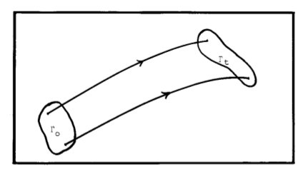
Figure 5.1: Volume-conserving flow in phase space.
An equivalent statement is that the Jacobian determinant of the transformation \( \langle q_1(0), \ldots, p_n(0)\rangle \mapsto \langle q_1(t), \ldots , p_n(t)\rangle \) is identically equal to unity:
\begin{equation} \frac{\partial(q_{1t},\ldots p_{nt})}{\partial(q_{10}\ldots q_{n0})} = \left| \begin{matrix} \frac{\partial q_{1t}}{\partial q_{10}}&\cdots & \frac{\partial p_{nt}}{\partial q_{10}}\\ \vdots&\ddots&\vdots\\ \frac{\partial q_{1t}}{\partial p_{n0}}&\cdots & \frac{\partial p_{nt}}{\partial p_{n0}}\\ \end{matrix}\right| = 1 \end{equation}
Problem (5.4). Prove that (5-9), (5-11), and (5-12) are equivalent statements. (Hint: See A. I. Khinchin, Mathematical Foundations of Statistical Mechanics, Chapter II.)
This result was termed by Gibbs the “Principle of conservation of extension-in—phase”, and is usually referred to nowadays as Liouville's theorem. An important advantage of considering the motion of a system referred to phase space (coordinates and momenta) instead of the coordinate—velocity space of the Lagrangian is that in general no such conservation law holds in the latter space (although they amount to the same thing in the special case where all the \(q_i\) are cartesian coordinates of particles and all forces are conservative in the sense of Problem 5.3).
Problem (5.5). Liouville's theorem holds only because of the special form of the Hamiltonian equations of motion, which makes the divergence (5-9) identically zero. Generalize it to a mechanical system whose state is defined by a set of variables \(\{x_1,x_2,\ldots,x_n\}\) with equations of motion for \(x_i(t)\): \begin{equation} \dot{x}_i(t) = f_i(x_1,\ldots,x_n),\qquad i=1,2,\ldots,n \end{equation} The jacobian (5-12) then corresponds to
\begin{equation} J(x_1(0),\ldots,x_n(0);t) \equiv \frac{\partial[x_1(t),\ldots, x_n(t)]}{\partial[x_1(0),\ldots,x_n(0)]} \end{equation}Prove that in place of Liouville's theorem \(J=1=\text{const.}\), we now have
\begin{equation} $J(t) = J(0)\,\exp\left[\int_0^t \sum_{i=1}^n \frac{\partial f[x_1(t),\ldots, x_n(t)]}{\partial x_i(t)} dt\right]. \end{equation}
2.3 The Structure Function
One of the essential dynamical properties of a system, which controls its thermodynamic properties, is the total phase volume compatible with various experimentally observable conditions. In particular, for a system in which the Hamiltonian and the energy are the same, the total phase volume below a certain energy \(E\) is
\begin{equation} \Omega(E) = \int \vartheta[E-H(q_i,p_i)] dq_i\ldots dp_n \end{equation}(When limits of integration are unspecified, we understand integration over all possible values of qi, pi.) In (5-16) , \(\vartheta(x)\) is the unit step function
\begin{equation} \vartheta(x) \equiv \begin{cases}1,&x>0\\ 0,&x<0\end{cases} \end{equation}The differential phase volume, called the structure function, is given by \begin{equation} \rho(E) = \frac{d\Omega}{dE} = \int \delta[E-H(q_i,p_i)] dq_1\ldots dp_n \end{equation} and it will appear presently that essentially all thermodynamic properties of the system are known if \(\rho(E)\) is known, in its dependence on such parameters as volume and mole numbers.
Calculation of \(\rho(E)\) directly from the definition (5-18) is generally very difficult. It is much easier to calculate first its Laplace transform, known as the partition function:
\begin{equation} Z(\beta) = \int_0^\infty e^{-\beta E} \rho(E)\, dE \end{equation}where we have assumed that all possible values of energy are positive; this can always be accomplished for the systems of interest by appropriately choosing the zero from which we measure energy. In addition, it will develop that full thermodynamic information is easily extracted directly from the partition function \(Z(\beta)\) , so that calculation of the structure function \(\rho(E)\) is unnecessary for some purposes.
Footnotes:
1 Edit: The set of solutions to an equation like f(X,x,t)= const. is called a level set. Here, Jaynes is saying that the quantities X, x, and t follow a “functional rule”, so the set of physically allowed combinations of X, x, and t in equilibrium states can be expressed as the level set of a function.
But not every function expresses a constraint relation; for some functions, you can specify two of the variables, and the third will still be undetermined. (For example, if f=X2+x2+t2-3, the level set f(X,x,t)=0 is a sphere, and specifying x=1, t=1 leaves you with two potential possibilities for X =± 1.)
A function like f has to possess one more propery in order for its level set to express a constraint relationship: it must be monotonic in each of its variables X, x, and t. In other words, the level set has to pass a sort of “vertical line test” for each of its variables.
2 Edit: The first equality comes from our requirement that \(dQ = T\,dS\). The second equality comes from the fact that \(dU = dQ - dW\) (the first law) and that \(dW = PdV\) in the case where the state has two degrees of freedom, pressure and volume.
3 Edit: A differential \(M(x,y)dx + N(x,y)dy\) is called exact if there is a scalar function \(\Phi(x,y)\) such that \(M = \frac{\partial \Phi}{\partial x}\) and \(N=\frac{\partial \Phi}{\partial y}\). If there is, Φ is called the potential function of the differential, Conceptually, this means that M(x,y)dx + N(x,y) dy is the derivative of a scalar potential and so consequently corresponds to a conservative field.
Even if there is no such potential function Φ for the given differential, it is possible to coerce an inexact differential into an exact one by multiplying by an unknown function \(\mu(x,y)\) (called an integrating factor) and requiring the resulting differential \(\mu M\, dx + \mu N\, dy\) to be exact.
To complete the analogy, here we have the differential \(dQ = dU + PdV\) (by the first law) which is not exact—conceptually, there is no scalar potential nor conserved quantity corresponding to \(dQ\). We have introduced a new differential \(dS = \frac{1}{T}dQ\), and we are searching for the temperature scale \(T(U,V)\) which makes \(dS\) exact (i.e. which makes \(S\) correspond to a conserved quantity). This means that \(\frac{1}{T}\) is playing the role of the integrating factor “μ” for the differential \(dQ\).
4 Note, however, that the second law has nothing to say about how rapidly this approach to equilibrium takes place.
5 Edit: See also, the Open Library page, where you can read and download Maxwell's book in a variety of formats.
6 Edit: Hilsch's paper is entitled The use of the expansion of gases in a centrifugal field as a cooling process.